Polymorphism – Allotropy
Polymorphism
– The occurrence of the same substance in more than one crystalline forms is known as Polymorphism.
– Polymorphism phenomenon is shown by both elements and compounds. In the case of elements the term allotropy is often used.
– The individual crystalline forms of an element are referred to as polymorphs or allotropes.
– Rhombic and monoclinic sulphur are two polymorphs or allotropes of sulphur.
– The polymorphic or allotropic forms of an element have distinct physical properties and constitute separate phases.
– Allotropy can be divided into three types : Enantiotropy, Monotropy and Dynamic allotropy.
(1) Enantiotropy
– In some cases one polymorphic form (or allotrope) can change into another at a definite temperature when the two forms have a common vapour pressure. This temperature is known as the transition temperature.
– One form is stable above this temperature and the other form below it.
– When the change of one form to the other at the transition temperature is reversible, the phenomenon is called enantiotropy and the polymorphic forms enantiotropes.
– For example, rhombic sulphur (α-Sulphur) on heating changes to monoclinic sulphur (β-Sulphur) at 95.6º C (transition temperature).
– Also, monoclinic sulphur, on cooling, again changes to rhombic sulphur at 95.6ºC. That is,
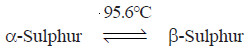
– Thus α-Sulphur and β-Sulphur are enantiotropic.
(2) Monotropy
– It occurs when one form is stable and the other metastable.
– The metastable changes to the stable form at all temperatures and the change is not reversible.
– Thus there is no transition temperature as the vapour pressures are never equal. This type of polymorphism is exhibited by phosphorus,
White phosphorus ⎯⎯→ Red phosphorus
– Another example is graphite and diamond, graphite being stable and diamond metastable, although the change is infinitely slow.
(3) Dynamic allotropy
– Some substances have several forms which can coexist in equilibrium over a range of temperature.
– The amount of each is determined by the temperature.
– The separate forms usually have different molecular formulae but the same empirical formula.
– This form of allotropy, known as dynamic allotropy, resembles enantiotropy in that it is reversible but there is no fixed transition point.
– An example of dynamic allotropy is provided by liquid sulphur which consists of three
allotropes Sμ, Sπ and Sλ.
Sμ ↔ Sπ ↔ Sλ
– These three forms of sulphur differ in molecular structure.
– Sλ is S8, Sπ is S4 while formula of Sμ is not known.
– The composition of the equilibrium mixture at 120ºC and 444.6ºC (b.p. of sulphur) is:
![]()
Experimental Determination of transtion point
– The temperature at which a polymorphic substance changes from one form to another, is known as the transition temperature or transition point.
– For example, rhombic variety of sulphur is converted to the monoclinic form of sulphur at 95.6º C at atmospheric pressure.
– The transition temperature in a particular case can be determined by measuring a change in physical properties such as colour, density, solubility, etc.
(1) Colour change
If a little mercury (II) iodide is placed in a melting point tube attached to a thermometer and heated in some form of apparatus (e.g., electrical heater), it is possible to record temperature at which the red mercury (II) iodide changes to the yellow form.
(2) Density change
– As rhombic sulphur changes to monoclinic sulphur, there is a decrease in density and, therefore, an increase in volume.
– The change in volume is employed to measure the transition temperature by using an apparatus known as Dilatometer shown in Fig below.
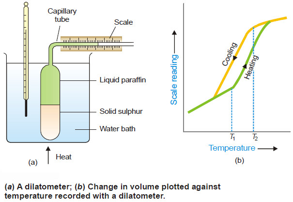
– Some powdered rhombic sulphur is placed in the glass bulb and liquid paraffin (an inert liquid) is introduced above the sulphur.
– The apparatus is then immersed in a heating water-bath, the temperature of which is raised.
– The scale reading and the temperature is recorded every minute.
– A plot of liquid level in the capillary against temperature gives a curve as in Fig(b).
– On cooling of the dilatometer, reverse changes take place but due to thermal lag the curve assumes the form shown in the figure.
– The transition temperature is taken as the mean of the respective temperatures where expansion starts (T1) and contraction begins (T2).
(3) Solubility change
– Two forms of the same substance have different solubilities but at the transition point they have
identical solubility.
– Thus if solubility-temperature graph is plotted for the two forms, it is found to
consist of two parts with a sharp break.
– While one part represents the solubility curve for one form, the second part represents that for the other.
– At the meeting point of the two curves, the solubility of the two forms is the same and it indicates the transition temperature.
– For example, in the diagram for the system sodium sulphate-water, the solubility curves of Na2SO4 (rhombic) and Na2SO4.10H2O meet at 32.2ºC.
– Thus 32.2ºC is the transition temperature where Na2SO4.10H2O changes to Na2SO4.
(4) Cooling curve method
– There is often an evolution or absorption of heat when one form passes to the other.
– Suppose that form A is converted into form B on heating.
– Now let B be allowed to cool and a curve obtained by plotting the temperature against the time.
– The otherwise steady curve has a distinct break at a temperature corresponding to the transition point because here heat is evolved from B.
– This method is suitable for determining the transition temperature between different hydrates of a salt or between a hydrate and an anhydrous salt (e.g., Na2SO4.10H2O to Na2SO4), or for different forms of a metal.