
Activity Coefficients : Definition, Equation, Examples, Properties
– In this topic, we will discuss Activity coefficients : Definition, Equation, Examples and Properties.
Activity Coefficients
– Chemists use a term called activity, a, to account for the effects of electrolytes on chemical equilibria.
– The activity, or effective concentration, of species X depends on the ionic strength of the medium and is defined by:
![]() (1)
(1)
– where aX is the activity of the species X, [X] is its molar concentration, and γX is a dimensionless quantity called the activity coefficient.
– The activity coefficient and thus the activity of X vary with ionic strength.
– If we substitute aX for [X] in any equilibrium-constant expression, we find that the equilibrium constant is then independent of the ionic strength.
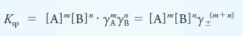
– To illustrate this point, if XmYn is a precipitate, the thermodynamic solubility product expression is defined by the equation:
![]() (2)
(2)
– Applying Equation (1) gives:
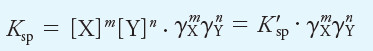
– In this equation, K’sp is the concentration solubility product constant, and Ksp is the thermodynamic equilibrium constant.
– The activity coefficients γX and γY vary with ionic strength in such a way as to keep Ksp numerically constant and independent of ionic strength (in contrast to the concentration constant, K’sp).
Properties of Activity Coefficients
– Activity coefficients have the following properties:
(1) The activity coefficient of a species is a measure of the effectiveness with which that species influences an equilibrium in which it is a participant.
– In very dilute solutions in which the ionic strength is minimal, this effectiveness becomes constant, and the activity coefficient is unity.
– Under these circumstances, the activity and the molar concentration are identical (as are thermodynamic and concentration equilibrium constants).
As the ionic strength increases, however, an ion loses some of its effectiveness, and its activity coefficient decreases.
– We may summarize this behavior in terms of Equations (1) and (2).
– At moderate ionic strengths, γX<1. As the solution approaches infinite dilution, however, γX→1, and thus, aX → [X] while K’sp → Ksp.
– At high ionic strengths ( μ > 0.1 M), activity coefficients often increase and may even become greater than unity.
– Because interpretation of the behavior of solutions in this region is difficult, we confine our discussion to regions of low or moderate ionic strength (that is, where μ ≤ 0.1 M).
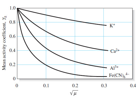
– The variation of typical activity coefficients as a function of ionic strength is shown in Figure:
(2) In solutions that are not too concentrated, the activity coefficient for a given species is independent of the nature of the electrolyte and dependent only on the ionic strength.
(3) For a given ionic strength, the activity coefficient of an ion decreases more dramatically from unity as the charge on the species increases.
– This effect is shown in Figure above.
(4) The activity coefficient of an uncharged molecule is approximately unity, no matter what the level of ionic strength.
(5) At any given ionic strength, the activity coefficients of ions of the same charge are approximately equal.
– The small variations among ions of the same charge can be correlated with the effective diameter of the hydrated ions.
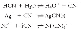
(6) The activity coefficient of a given ion describes its effective behavior in all equilibria in which it participates.
– For example, at a given ionic strength, a single activity coefficient for cyanide ion describes the influence of that species on any of the following equilibria:
The Debye-Hückel Equation
– In 1923, P. Debye and E. Hückel used the ionic atmosphere model, to derive an equation that permits the calculation of activity coefficients of ions from their charge and their average size.
– This equation, which has become known as the Debye-Hückel equation, takes the form:
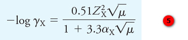
where
γX = activity coefficient of the species X
ZX = charge on the species X
μ = ionic strength of the solution
αX = effective diameter of the hydrated ion X in nanometers (1029 m)
– The constants 0.51 and 3.3 are applicable to aqueous solutions at 25°C.
– Other values must be used at other temperatures.
– Unfortunately, there is considerable uncertainty in the magnitude of αX in Equation (5).
– Its value appears to be approximately 0.3 nm for most singly charged ions. For these species, then, the denominator of the Debye-Hückel equation simplifies to approximately ![]()
– For ions with higher charge, αX may be as large as 1.0 nm. This increase in size with increase in charge makes good chemical sense.
– The larger the charge on an ion, the larger the number of polar water molecules that will be held in the solvation shell around the ion.
– The second term of the denominator is small with respect to the first when the ionic strength is less than 0.01 M.
– At these ionic strengths, uncertainties in αX have little effect on calculating activity coefficients.
Kielland has estimated values of αX for numerous ions from a variety of experimental
data.
– His best values for effective diameters are given in the following Table:
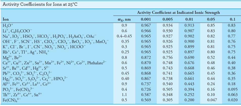
– Also presented are activity coefficients calculated from Equation (5) using these values for the size parameter.
– It is unfortunately impossible to determine experimentally single-ion activity coefficients such as those shown in Table above because experimental methods give only a mean activity coefficient for the positively and negatively charged ions in a solution.
– In other words, it is impossible to measure the properties of individual ions in the presence of counter-ions of opposite charge and solvent molecules.
– We should point out, however, that mean activity coefficients calculated from the data in Table above agree satisfactorily with the experimental values.
Mean Activity Coefficients
– The mean activity coefficient of the electrolyte AmBn is defined as:
![]()
– The mean activity coefficient can be measured in any of several ways, but it is impossible experimentally to resolve this term into the individual activity coefficients for γA and γB.
– For example, if
– we can obtain Ksp by measuring the solubility of AmBn in a solution in which the electrolyte concentration approaches zero (that is, where both γA and γB → 1).
– A second solubility measurement at some ionic strength μ1 gives values for [A] and [B].
– These data then permit the calculation of ![]() for ionic strength μ1.
for ionic strength μ1.
– It is important to understand that this procedure does not provide enough experimental data to permit the calculation of the individual quantities γA and γB and that there appears to be no additional experimental information that would permit evaluation of these quantities.
– This situation is general, and the experimental determination of an individual activity coefficient is impossible
Example (1):
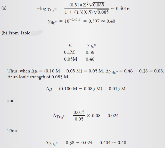
(a) Use Equation (5) to calculate the activity coefficient for Hg2+ in a solution that has an ionic strength of 0.085 M. Use 0.5 nm for the effective diameter of the ion.
(b) Compare the value obtained in (a) with the activity coefficient obtained by linear interpolation of the data in Table above for coefficients of the ion at ionic strengths of 0.1 M and 0.05 M.
Solution:
– Based on agreement between calculated and experimental values of mean ionic activity coefficients, we can infer that the Debye-Hückel relationship and the data in Table above give satisfactory activity coefficients for ionic strengths up to about 0.1 M. Beyond this value, the equation fails, and we must determine mean activity coefficients experimentally.
Equilibrium Calculations Using Activity Coefficient
– Equilibrium calculations using activities produce results that agree with experimental data more closely than those obtained with molar concentrations.
– Unless otherwise specified, equilibrium constants found in tables are usually based on activities and are thus thermodynamic constants.
– The examples that follow illustrate how activity coefficients from Table above are used with thermodynamic equilibrium constants.
Example (2): Use activities to calculate the hydronium ion concentration in a 0.120 M solution of HNO2 that is also 0.050 M in NaCl. What is the relative percent error incurred by neglecting activity corrections?
Solution:
The ionic strength of this solution is:
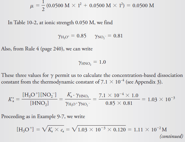
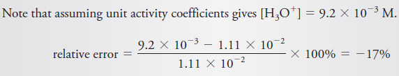
– In this example, we assumed that the contribution of the acid dissociation to the ionic strength was negligible.
– In addition, we used the approximate solution for calculating the hydronium ion concentration.
Omitting Activity Coefficients in Equilibrium Calculations
– We normally neglect activity coefficients and simply use molar concentrations in
applications of the equilibrium law.
– This approximation simplifies the calculations and greatly decreases the amount of data needed.
– For most purposes, the error introduced by the assumption of unity for the activity coefficient is not large enough to lead to false conclusions.
– The preceding examples illustrate, however, that disregarding activity coefficients may introduce significant numerical errors in calculations of this kind.
– Be alert to situations in which the substitution of concentration for activity is likely to lead to maximum error.
– Significant discrepancies occur when the ionic strength is large (0.01 M or larger) or when the participating ions have multiple charges (see Table above).
– With dilute solutions (μ <0.01 M) of nonelectrolytes or of singly charged ions, mass-law calculations using concentrations are often reasonably accurate. When, as is often the case, solutions have ionic strengths greater than 0.01 M, activity corrections must be made.
– Computer applications such as Excel greatly reduce the time and effort required to make these calculations.
– It is also important to note that the decrease in solubility resulting from the presence of an ion common to the precipitate (the common-ion effect) is in part counteracted by the larger electrolyte concentration of the salt containing the common ion.
Reference: Fundamentals of analytical chemistry / Douglas A. Skoog, Donald M. West, F. James Holler, Stanley R. Crouch. (ninth edition) , 2014 . USA
nice thank you